Image Preprocessing for Short Term Solar Irradiance Forecasting

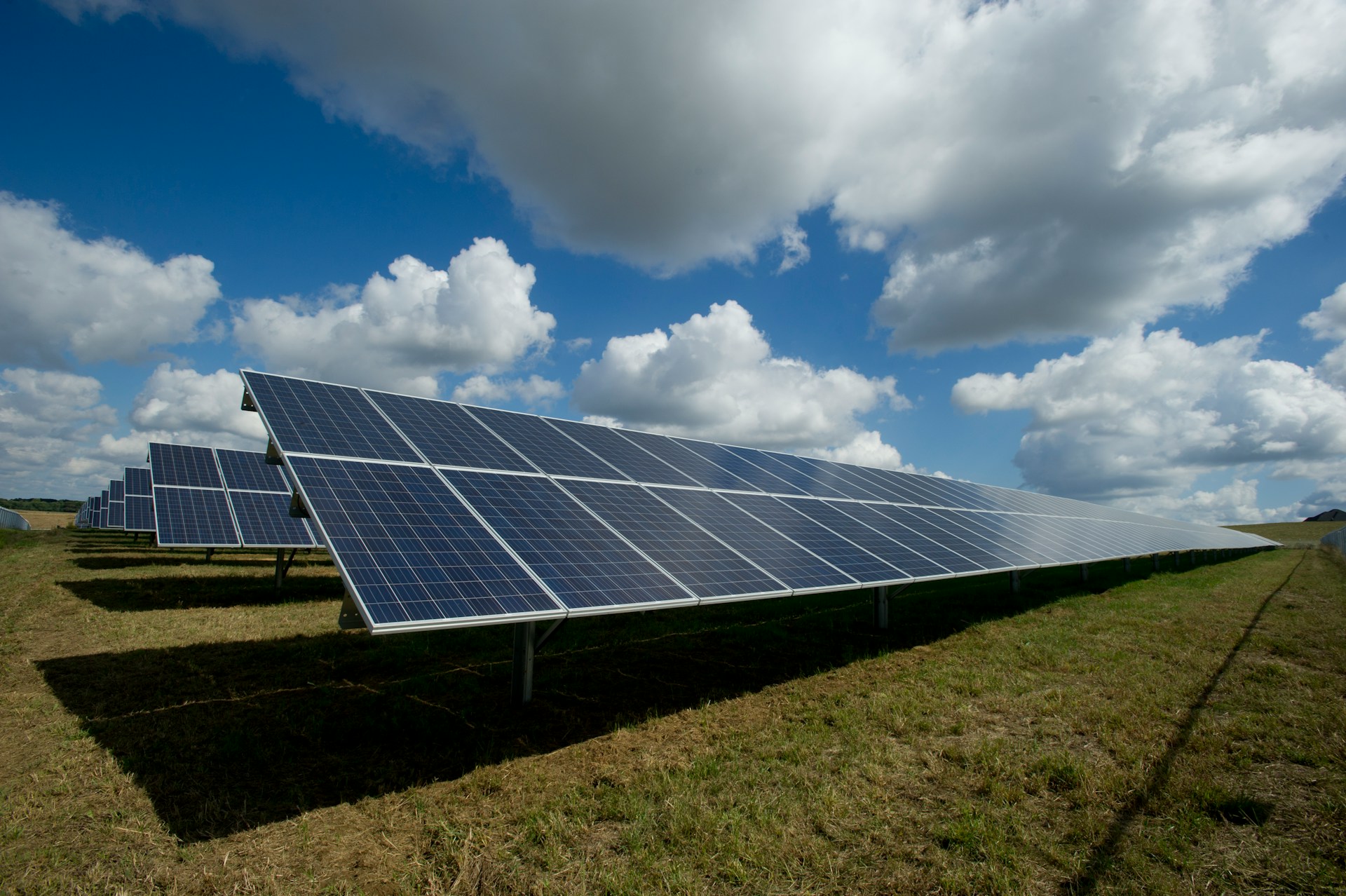
Photovoltaic (PV) systems are a popular, if not the most popular, alternative means of electricity generation and the energy they generate is directly proportional to solar irradiance. Solar irradiance is a measure of the surface power density (power per unit area - W/m2) received from the Sun via electromagnetic radiation in the wavelength range of the measuring instrument. There are various measured types of solar irradiance which include - total solar irradiance (TSI), Global horizontal irradiance (GHI), Diffuse horizontal irradiance (DHI), amongst others. The study of solar irradiance has several important applications; however, this post focuses only on the prediction of energy generation from solar power plants. Forecasting solar irradiance is therefore important for planning the power output of these PV systems [1].
Solar Irradiance Forecasting for South Africa
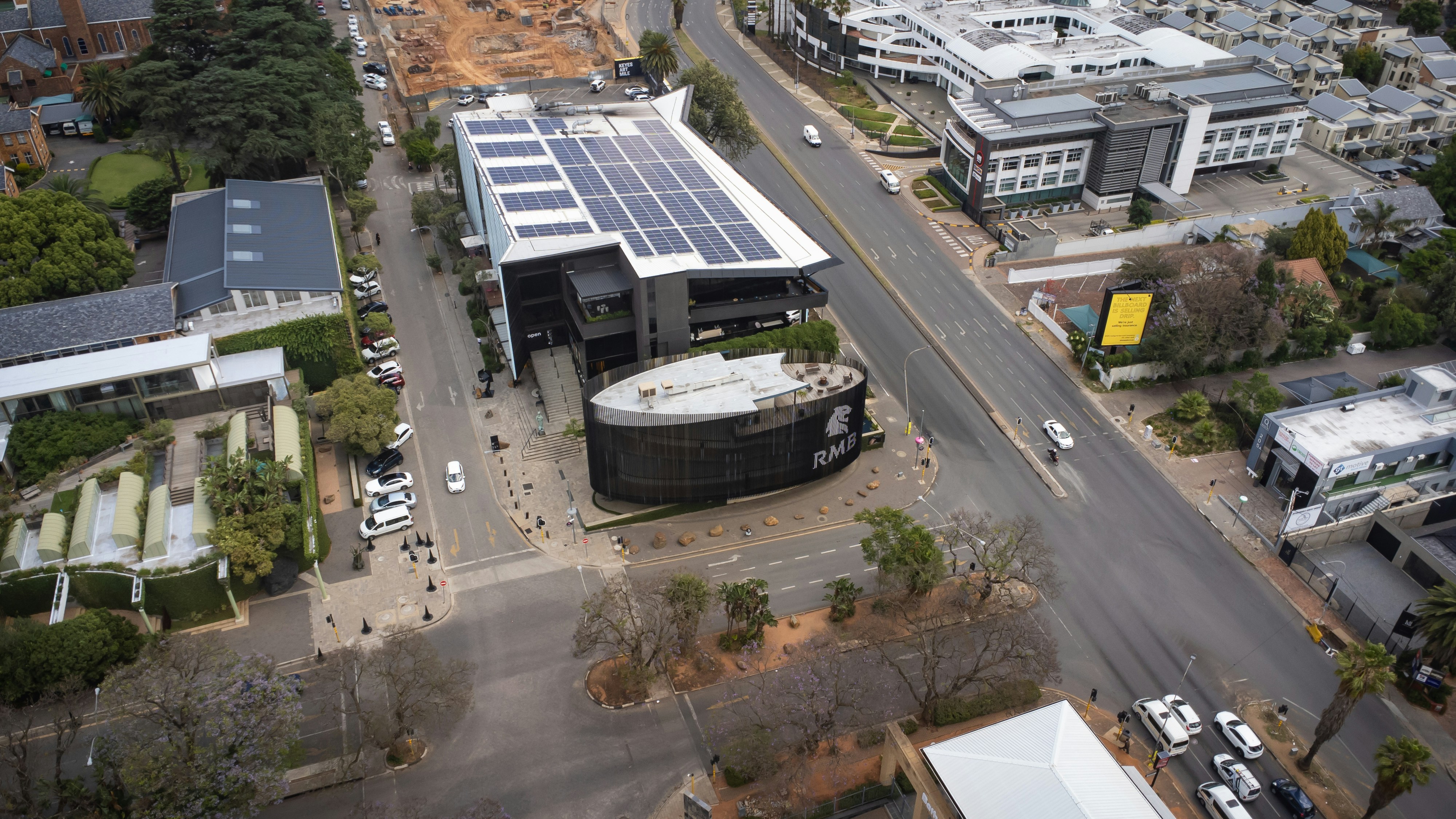
South Africa’s currency electricity system has struggled in the recent past ever since the beginning of load shedding in 2007, this has spurred the rapid growth of photovoltaic systems as the public and private sector look to address the unstable electricity situation in the country. Rooftop solar photovoltaic market in South Africa is estimated at 2.31 gigawatt and is expected to reach 3.40 gigawatt by 2030. However, there needs to be work done to avoid grid congestion since South Africa’s grid system was designed for coal energy rather than renewable sources such as solar and wind. Therefore, solar generation prediction is a crucial tool that is used to provide grid stability and economic planning, to manage the variable output from the increasing solar capacity.
Machine Learning Solar Irradiance Forecasting Techniques
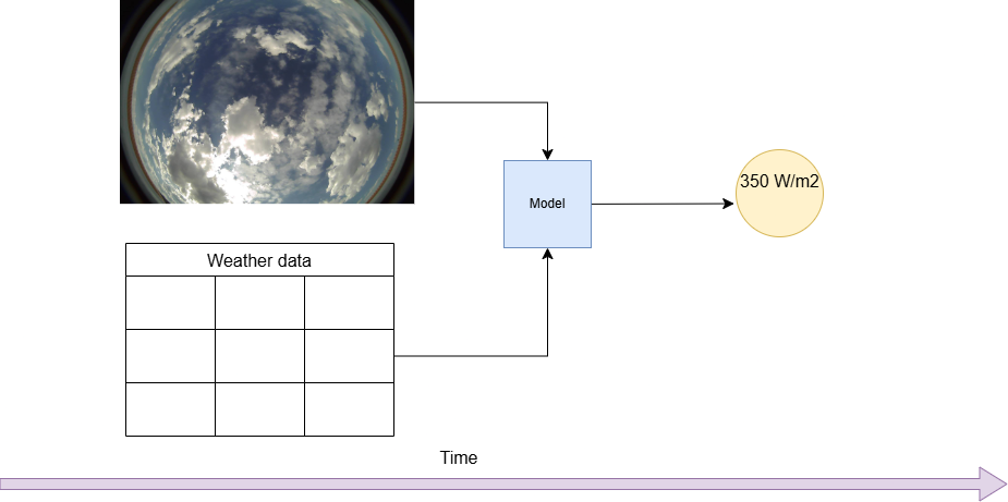
The World Meteorological Organization (WMO) defines nowcasting, short-range forecasting, as the description of the current weather situation up to 6 hours ahead in the future time horizon. For solar energy, nowcasting is usually focused on future time scales of up to 20 min - enabling grid managers to effectively react under real-time constraints. Currently, solar irradiance nowcasting makes use of all-sky images due to their wide angle view and with their frequent retrieval enable cloud movement can be monitored. Currently, there are 3 approaches used for cloud detection in solar nowcasting literature:
1. Fixed or adaptive thresholds applied to colour channels
2. Clear sky library (CSL) to distinguish between clear and cloud sky based on the solar position and atmospheric constituents
3. Machine learning for deriving representations from all-sky images
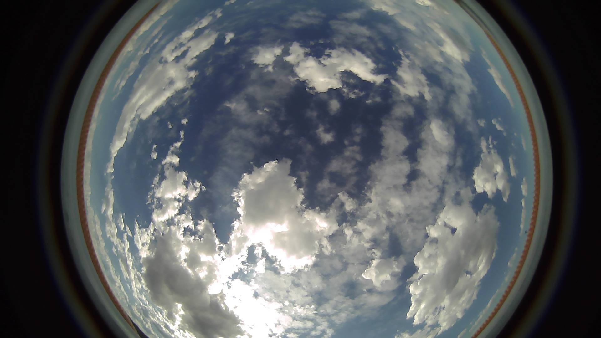
In this blog, we will go through the first stages of pre-processing all-sky images before they can be utilized by advanced algorithms such as CNNs or Vision Transformers, to provide multimodal (sky images + meteorological data) solar irradiance nowcasting. Sky images make use of fisheye lenses since the ultra-wide-angle lenses capture the entire dome of the sky (180 degrees) in a single shot. The images have a distinctive panoramic look which makes them ideal for weather monitoring.
CloudCV 10-Second Sky Images and Irradiance Dataset
The CloudCV 10-Second Sky Image and Irradiance Dataset contains sky images and irradiance measurements recorded every 10 seconds during daylight hours for 90 days between September 5th to December 3rd, 2019. The dataset was collected at the National Renewable Energy Laboratory (NREL) Solar Radiation Research Laboratory (SRRL) mesa-top campus in Golden, Colorado, USA. The instruments used include an ELP 180 degree Fisheye Lens Wide Angle USB Camera webcam and a co-located LICOR LI200 pyranometer. The images used in this subset are sky images and irradiance data for 2019-09-07. More information available - https://data.nrel.gov/submissions/248.
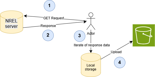
Subsets of the dataset have been made available by the NREL research team on the webpage for this project. The subsets are in tar.gz format, we make a GET request to the specific subset and write the content to local storage.
import boto3
import requests
from getpass import getpass

# setup AWS credentials
aws_access_key_id = getpass('Enter your access key ID')
aws_secret_access_key = getpass('Enter your secret access key')
region_name = getpass('Enter your AWS region')

# set boto3s3client
client = boto3.client('s3',
                      aws_access_key_id=aws_access_key_id,
                      aws_secret_access_key=aws_secret_access_key,
                      region_name=region_name)
# configuration
bucket_name = "BUCKET_NAME" # bucket name removed for privacy
dataset_url = "https://data.nrel.gov/system/files/248/1727737056-2019_09_07.tar.gz"
local_file = "solar_dataset.tar.gz"
s3_key = "KEY" # key is the name of path in bucket

# make GET request to download data to local storage
print("Downloading dataset...")
response = requests.get(dataset_url, stream=True)
with open(local_file, "wb") as f:
    for chunk in response.iter_content(chunk_size=8192):
        f.write(chunk)

!tar -xzvf "solar_dataset.tar.gz" -C "solar_dataset/" # execute in seperate cell to unzip content
from pathlib import Path
# setup pathlib instance of images dir
dir = 'solar_dataset/images'
dir = Path(dir)
files_folders = [item for item in dir.iterdir()]
print(len(files_folders))

# upload all images to s3
for item in files_folders:
  item_path_str = str(item)
  item_file_name = item_path_str.split("/")[-1]
  client.upload_file(item_path_str, bucket_name, f"{s3_key}/images/{item_file_name}")
  print(f"uploaded to s3://{bucket_name}/{s3_key}/{item_file_name}")
print("DONE")
Viewing and pre-processing the Files on S3
Now that the images are on S3, the next steps will be to view them and begin the pre-processing - removal of fisheye distortion from the images. We will define several helper functions to assist us during the process. This example made use of S3FS library which enables us to interact with s3 objects as if they were local files. Boto3 will be extensively used as we are interacting with AWS in Python.
# import necessary libraries
import torch
import pandas as pd
import numpy as np
import matplotlib.pyplot as plt
from PIL import Image
from s3pathlib import S3Path
import io
from tqdm.auto import tqdm
import defisheye
import s3fs
import cv2
import random

# helper functions
def create_authenticated_file_system(aws_access_key_id, aws_secret_access_key):
  """ Creates an authenticated file system with valid AWS credentials enabling us to treat s3 as a local file system."""
  fs = s3fs.S3FileSystem(key=aws_access_key_id, secret=aws_secret_access_key,anon=False)
  fs.invalidate_cache()
  return fs
#
def get_s3_img_paths(client,bucket_name, prefix):
  """Return a list containing the uri of each obect(image in this instance) in bucket location."""
  path_list = []
  paginator = client.get_paginator("list_objects_v2")
  for page in paginator.paginate(Bucket=bucket_name, Prefix=prefix):
    for obj in page.get("Contents", []):
      path_list.append(f"s3://{bucket_name}/"+obj["Key"])
  return path_list

# get all the images in directory
s3_image_path_list = get_s3_img_paths(client=client, bucket_name=bucket_name, prefix=image_key)
print(f"Number of images found in directory : {len(s3_image_path_list)}")
print(f"The bucket contains {(len(s3_image_path_list)/number_of_images_dataset):.2%} of the CloudCV 10-Second Sky Images and Irradiance Dataset")

sample_img_path = "s3://{bucket_name}/{key}/UTC-7_2019_09_07-06_40_18_651869.jpg" # key specifies location in the bucket
fs = create_authenticated_file_system(aws_access_key_id,aws_secret_access_key)
with fs.open(f"{sample_img_path}","rb") as file:
    img = Image.open(io.BytesIO(file.read()))
    img_array = np.asarray(img)
plt.imshow(img_array)
plt.title(f"{sample_img_path}")
plt.axis(False)
Day or Night?
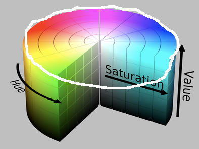
There are around 4557 images in this subset, which is around 1% of the images in the full dataset. Although the images are collected during daylight hours, in some of the images the sun has set and it is practically night. We need to be able to separate these images from the others where we can capture cloud position and movement. To do this we use an agricultural method of determining whether the image is day or night. This is done using the cv2 library to analyse the image’s brightness or colour characteristics. We set a threshold for brightness values that range from 0 (black) to 255 (full intensity). The code below will convert the Blue-Green-Red format to Hue-Saturation-Value format.
def day_or_night_classifier(img_bytes, threshold=50):
np_1d_array = np.frombuffer(img_bytes, dtype="uint8")
img = cv2.imdecode(np_1d_array, cv2.IMREAD_COLOR) # load image into default BGR format
if img is None:
raise ValueError("Error: Could not load image")
# convert image to HSV colour space
hsv_img = cv2.cvtColor(img, cv2.COLOR_BGR2HSV)
# get the brightness channel (Valueu)
_,_,v_channel = cv2.split(hsv_img)
# calculate average_brighness
average_brightness = v_channel.mean()
print(f"calculated average brigthness - {average_brightness:.2f}")
if average_brightness > threshold:
return "Day"
else:
return "Night"
# test function
with fs.open(f"{sample_img_path}","rb") as file:
img_bytes = io.BytesIO(file.read()).getbuffer()
result = day_or_night_classifier(img_bytes)
print(result)
# iterate through the dataset to split images into day and night sets
img_dict = {
"day_images":[],
"night_images":[]
}
for img_path in s3_image_path_list:
with fs.open(f"{img_path}","rb") as file:
# convert image to bytes
img_bytes = io.BytesIO(file.read()).getbuffer()
# classify image into day and night
result = day_or_night_classifier(img_bytes)
print(f"{img_path} classified - {result}")
if result == "Day":
# update img dict
img_dict["day_images"].append(img_path)
else:
# update img dict
img_dict["night_images"].append(img_path)
day_images, len_day_images = img_dict["day_images"],len(img_dict["day_images"])
night_images, len_night_images = img_dict["night_images"],len(img_dict["night_images"])
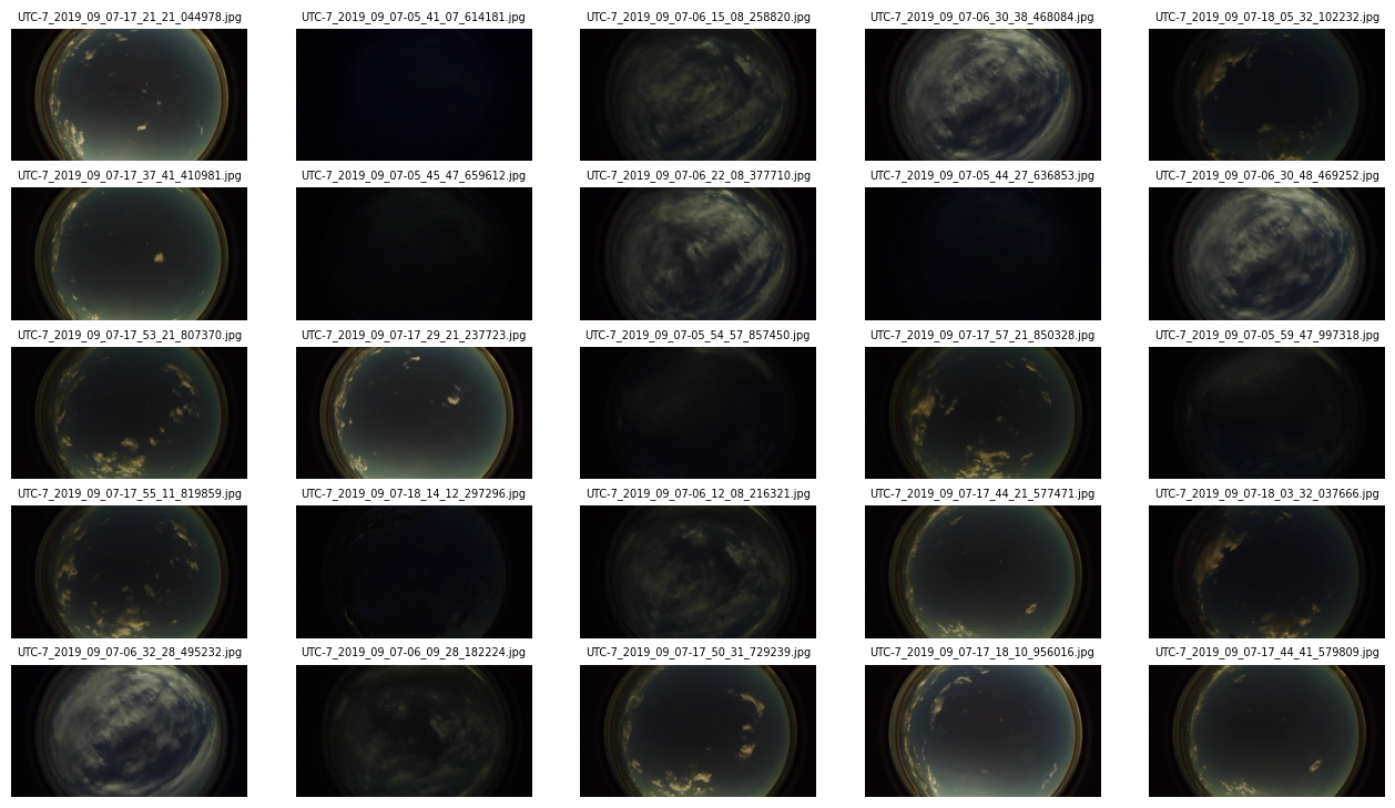
print(f"Length of day images - {len(day_images)}\nlength of night images - {len(night_images)}")View Day Images
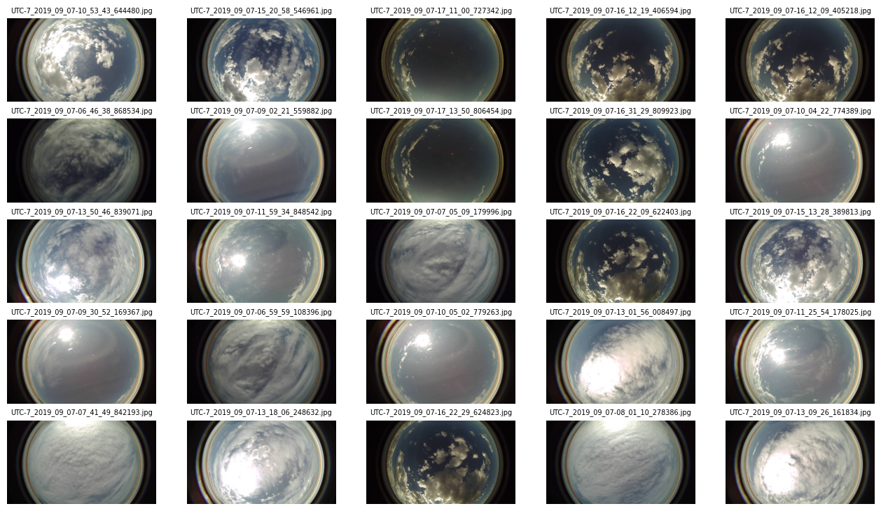
Let us view the images that our classifier classified as day images.
# view day images
random.seed(25)
fig = plt.figure(figsize=(16,9))
rows, cols = 5, 5
for i in range(1, rows*cols+1):
  # get random index
  random_index = random.randint(0, len_day_images-1)
  random_img_path = day_images[random_index]
  with fs.open(f"{random_img_path}","rb") as file:
    img = Image.open(io.BytesIO(file.read()))
    img_array = np.asarray(img)
    fig.add_subplot(rows, cols, i)
    plt.imshow(img)
    plt.title(random_img_path.split("/")[-1], fontsize=7, wrap=True)
    plt.axis(False)
View Night Images
Let us view the images that our classifier classified as night images.
# view night images
random.seed(25)
fig = plt.figure(figsize=(16,9))
rows, cols = 5, 5
for i in range(1, rows*cols+1):
  # get random index
  random_index = random.randint(0, len_night_images-1)
  random_img_path = night_images[random_index]
  with fs.open(f"{random_img_path}","rb") as file:
    img = Image.open(io.BytesIO(file.read()))
    img_array = np.asarray(img)
    fig.add_subplot(rows, cols, i)
    plt.imshow(img)
    plt.title(random_img_path.split("/")[-1], fontsize=7, wrap=True)
    plt.axis(False)
Lens Distortion with Defisheye
According to the paper that accompanied this data, the authors used the following pre-processing steps:
1. downsize the images to 500x500
2. perform spherical coordinate transformation to map fish-eye images to undistorted images - simply put, remove the fish eye effect on the images.
To do this, we used the Defisheye python module.

def remove_fisheye_distortion(img, dtype, format, fov, pfov):
  obj = defisheye.Defisheye(img, dtype=dtype, format=format, fov=fov, pfov=pfov)
  return obj.convert()

def image_transformation_pipeline(img_path:str, res_shape:tuple=(500,500),
                                  dtype:str="linear", format:str="fullframe",
                                  fov:int=180, pfov:int=110):
  with fs.open(f"{img_path}","rb") as file:
    # original image
    img = Image.open(io.BytesIO(file.read()))
    img_array = np.asarray(img)
    # perform rescale
    img_array_scaled = np.asarray(img.resize(res_shape, Image.BILINEAR))
    # perform fisheye distortion removal
    img_processed = remove_fisheye_distortion(img_array_scaled,dtype=dtype, format=format, fov=fov, pfov=pfov)
  return img_processed

dtype = "linear"
format = "fullframe"
fov = 180
pfov = 110

sample_img_path = "image uri" # removed for privacy

fig = plt.figure(figsize=(12,9))
rows, cols = 3,1
with fs.open(f"{sample_img_path}","rb") as file:
  # original image
  img = Image.open(io.BytesIO(file.read()))
  img_array = np.asarray(img)
  fig.add_subplot(rows, cols, 1)
  plt.imshow(img_array)
  plt.title(sample_img_path.split("/")[-1] +f"- {img_array.shape}", fontsize=7, wrap=True)
  plt.axis(False)
  # rescaled to 500 x 500
  res_shape = (500, 500)
  img_array_scaled = np.asarray(img.resize(res_shape, Image.BILINEAR))
  fig.add_subplot(rows, cols, 2)
  plt.imshow(img_array_scaled)
  plt.title(sample_img_path.split("/")[-1]+f"- {img_array_scaled.shape}", fontsize=7, wrap=True)
  plt.axis(False)
  # fish eye removal
  img_processed = remove_fisheye_distortion(img_array_scaled,dtype=dtype, format=format, fov=fov, pfov=pfov)
  fig.add_subplot(rows, cols, 3)
  plt.imshow(img_processed)
  plt.title(sample_img_path.split("/")[-1]+ f" - {img_processed.shape}", fontsize=7, wrap=True)
  plt.axis(False)
Apply Transformation to Entire Dataset
After validating that the transformation function works, next step is to apply it to both day and night images.
image_key = "processed/day_images/"
for path in day_images:
  # get image name to use with key
  img_name = path.split("/")[-1]
  print(img_name)
  # get processed image
  processed_img = image_transformation_pipeline(img_path=path)
  # convert image array to PIL image object
  image = Image.fromarray(processed_img)
  # save image to in-memory buffer as jpeg
  buffer = io.BytesIO()
  image.save(buffer, format="JPEG")
  buffer.seek(0)
  client.upload_fileobj(buffer, bucket_name, image_key+f"{img_name}",ExtraArgs={'ContentType': 'image/jpeg'})
  print("uploaded "+image_key+f"{img_name}")

# night images
image_key = "processed/night_images/"
for path in night_images:
  # get image name to use with key
  img_name = path.split("/")[-1]
  print(img_name)
  # get processed image
  processed_img = image_transformation_pipeline(img_path=path)
  # convert image array to PIL image object
  image = Image.fromarray(processed_img)
  # save image to in-memory buffer as jpeg
  buffer = io.BytesIO()
  image.save(buffer, format="JPEG")
  buffer.seek(0)
  client.upload_fileobj(buffer, bucket_name, image_key+f"{img_name}",ExtraArgs={'ContentType': 'image/jpeg'})
  print("uploaded "+image_key+f"{img_name}")


# view random images with transformation applied
# view day images
random.seed(25)
fig = plt.figure(figsize=(16,16))
rows, cols = 5, 5
for i in range(1, rows*cols+1):
  # get random index
  random_index = random.randint(0, len(night_images_uploaded)-1)
  random_img_path = night_images_uploaded[random_index]
  # print(random_img_path)
  with fs.open(f"{random_img_path}","rb") as file:
    img = Image.open(io.BytesIO(file.read()))
    img_array = np.asarray(img)
    fig.add_subplot(rows, cols, i)
    plt.imshow(img)
    plt.title(random_img_path.split("/")[-1], fontsize=7, wrap=True)
    plt.axis(False)
Next Steps
1. Improve day/night image classifier to have a more intelligent method for determining day or night in the images.
2. Feature Extraction: Extract sky condition features from images, such as cloud coverage, cloud types, optical depth, and colour histograms (RGB channels, red-to-blue ratios). These capture the cloud motion and opacity critical for irradiance variability.
3. Data Augmentation and Pre-processing: Apply augmentations like rotation, flipping, brightness adjustments, and noise addition to increase dataset robustness against varying lighting. The images need to be sequenced temporally for short-term forecasting.
References
1. Forecasting the short-term solar irradiance of a fixed tilt 75 MW Photovoltaic plant in South Africa - https://www.sasec.org.za/full_papers/44.pdf
2. CloudCV 10-Second Sky Images and Irradiance Dataset - https://data.nrel.gov/submissions/248
3. Nowcasting Solar Irradiance Components Using a Vision Transformer and Multimodal Data from All-Sky Images and Meteorological Observations - https://doi.org/10.3390/en18092300